|
Information
Results
Resources
Our partners
|
|
|
|
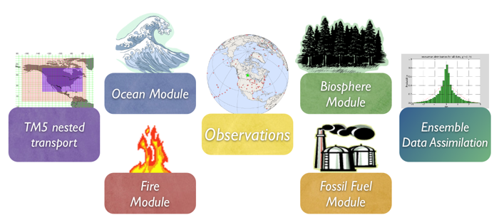
To learn more about a CarbonTracker Europe component, click on one of the above images.
Or download the full PDF version for convenience.
|
|
1. Introduction
The biospheric component of the carbon cycle consists of all the carbon stored in 'biomass' around us. This includes trees, shrubs, grasses, carbon within soils, dead wood, and leaf litter. Such reservoirs of carbon can exchange CO2 with the atmosphere. Exchange starts when plants take up CO2 during their growing season through the process called photosynthesis (uptake). Most of this carbon is released back to the atmosphere throughout the year through a process called respiration (release). This includes both the decay of dead wood and litter and the metabolic respiration of living plants. Of course, plants can also return carbon to the atmosphere when they burn, as described here. Even though the yearly sum of uptake and release of carbon amounts to a relatively small number (a few petagrams (one Pg=1015 g)) of carbon per year, the flow of carbon each way is as large as 120 Pg each year. This is why the net result of these flows needs to be monitored in a system such as ours. It is also the reason we need a good physical description (model) of these flows of carbon. After all, from the atmospheric measurements we can only see the small net sum of the large two-way streams (gross fluxes). Information on what the biospheric fluxes are doing in each season, and in every location on Earth is derived from a specialized biosphere model, and fed into our system as a first guess, to be refined by our assimilation procedure.
2. Detailed Description
The biosphere model currently used in CarbonTracker is the Simple-Biosphere-Model-Carnegie-Ames Stanford Approach (SiBCASA) biogeochemical model. This model calculates global carbon fluxes using input from weather models to drive biophysical processes, as well as satellite observed Normalized Difference Vegetation Index (NDVI) to track plant phenology. The version of SiBCASA model output used so far was driven by year specific weather and satellite observations, and including the effects of fires on photosynthesis and respiration (see van der Velde et al., [2014], van der Werf et al., [2006] and Giglio et al., [2006]). This simulation gives 1x1 degree global fluxes on a 10-minute time resolution, which we average to monthly means for further processing.
3-Hourly Net Ecosystem Exchange (NEE) is derived directly from Gross Primary Production (GPP) and ecosystem respiration (RE) from SiBCASA.
3. Further Reading
- van der Velde, I. R. et al. (2013), Biosphere model simulations of interannual variability in terrestrial 13C/12C exchange, Global Biogeochemical Cycles, 27(3), 637-649.
- van der Velde, I. R. et al. (2014), Terrestrial cycling of 13CO2 by photosynthesis, respiration, and biomass burning in SiBCASA , Biogeosciences, 11, 6553-6571.
- Schaefer, K. et al. (2008), Combined simple biosphere/Carnegie-Ames-Stanford approach terrestrial carbon cycle model. Journal of Geophysical Research: Atmospheres , 113(G3)
- Olsen and Randerson (2004), Differences between surface and column atmospheric CO2 and implications for carbon cycle research, Journal of Geophysical Research: Atmospheres, 109, D2, 27
- van der Werf, G.R. et al. (2006), Interannual variability in global biomass burning emissions from 1997 to 2004, Atm. Chem. Phys., 6(11), 3423-3441
|
|